How to Read S-Parameters: What S11 and S21 Tell You About Your PCB Layout

Anyone dealing with the design of high-speed PCBs, RF circuits or suffering signal integrity problems will encounter S-parameters (Scattering Parameters) sooner or later. As soon as the first frequency domain simulations or network analyzer measurements are done, waveforms such as so called S₁₁ and S₂₁ will appear for the engineer. But what can we actually get from them while working on a correct layout? And what exactly do these curves tell us about the behaviour of the PCB layout?

This is often where the uncertainty begins. Generally speaking, many people have an understanding that a low S₁₁ value and the highest possible S₂₁ value are desirable for a good signal transmission. But that doesn’t explain why the curves change even with small layout modifications. For example, what will happen with them when a trace becomes significantly longer? Why do reflections increase when the impedance changes? And what influence do the parameters like trace width, the height of the dielectric or its dielectric constant do have?

In this article, We’d like to illustrate these relationships not through detailed mathematical derivation but by using simple simulations and explaining the results and the relationships. The basis for this should be a microstrip PCB transmission line in which various parameters will be systematically varied. Among other factors, the analysis examines in particular the TL length, the TL impedance with values of 30 Ω, 50 Ω and 75 Ω, the TL trace width, the height of the dielectric and the dielectric constant of the PCB material.

In this process, only a single parameter is adjusted at a time, all other values remain unchanged. This makes it relatively easy to identify which change is dominantly responsible for the respective behavior of S11 and S₂₁.
The goal is not to derive a complete theory of scattering parameters. Instead, the goal is to develop a practical understanding of how S₁₁ and S₂₁ can be interpreted and what conclusions can be drawn from them regarding structures in the PCB layout. Layout engineers who understand why a curve changes can evaluate subsequent simulation- and/or measurement results more quickly and identify more effectively the possible root causes within the PCB layout.

1. What exactly do S-parameters mean?

Before we look at the simulation results, we should first clarify what S-parameters are all about. When a signal enters a PCB interconnect (trace), it should ideally reach the other end without attenuation or reflection. In practice, losses and reflections affect the transmission. S-parameters can be used to describe how a PCB trace—or, more generally, the entire transmission channel—affects the transmitted signal.

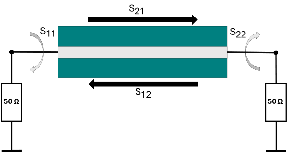
S-parameters can be used to describe what portion of the signal is transmitted and what amount is reflected. For a two-port network, there are a total of four S-parameters: S₁₁, S₂₁, S₁₂, and S₂₂.

S₂₁: How much of the signal arrives at the receiver?

S₂₁ describes the transmission from the input to the receiver. This parameter indicates what proportion of the input signal reaches the end of the line.

S₂₁ is typically expressed in decibels (dB). The closer the value is to 0 dB, the lower the transmission losses are. An ideal value of 0 dB would mean that the signal is transmitted without any attenuation.

However, various losses occur in a real PCB trace. These include, for example:

• ohmic losses in the conductor
• dielectric losses
• radiation
• reflections at impedance steps.

The more pronounced these effects are, the lower S₂₁ becomes. A decreasing S₂₁ value thus indicates that a smaller portion of the input signal reaches the output.

S₁₁: How much of the signal is reflected at the Input?

S₁₁ describes the reflection at the input of the transmission line. If the impedance of the trace does not match the reference impedance of the connected system or if there are impedance discontinuities along the trace, part of the signal will be reflected back to the source.

S11 is also usually expressed in decibels. The rule is: The smaller the value, the lower the reflection and the better the matching.

A simple example illustrates the relationship:

If a 50-Ω line is operated in a 50-Ω system, the line and the system are perfectly matched. As a result, no part of the signal is reflected, and S₁₁ would ideally be -∞.

If, on the other hand, the line impedance deviates from 50 Ω, a mismatch occurs. A larger portion of the signal will be reflected back. The S₁₁ value therefore becomes less negative and approaches 0 dB.

What do S₁₂ and S₂₂ describe?

In addition to S₁₁ and S₂₁ there are two other S-parameters.

S₁₂ describes the transmission in the opposite direction, means from the output back to the input. S₂₂ indicates the reflection at the output of the line.

For a passive and reciprocal PCB transmission line, the following applies:

• S₂₁ equals S₁₂.
• For a symmetrical configuration with identical reference impedances, S₁₁ also equals S₂₂.

In the following sections, we will examine how these two parameters will change when individual properties of the PCB structure—in this case, a PCB microstripline—are modified.

2. An Experiment with an ideal Transmission Line: The Influence of Length and Impedance

Before we examine real PCB microstrips with various trace widths, dielectric thicknesses and material properties, we will deliberately begin with an ideal transmission line example.

But what does “ideal” mean in this context? An ideal line is considered to be “lossless”. It comprises neither conductor losses nor dielectric losses.

This simplification allows us to focus initially on two fundamental questions: How does the line length affect the S-parameters? And what happens if the characteristic impedance of the line does not match the reference impedance of the ports?

In the first investigation, we examine three ideal lossless transmission lines. All with a characteristic impedance value of 50 Ω but different line length:

• 10 mm – blue
• 30 mm – red
• 60 mm – green

The reference impedance of both ports is also 50 Ω. This means that all three transmission lines are ideally matched to the system. Therefore, regardless of their length,  no reflections should occur in theory. In the linear scale, S₁₁ equals zero. In a logarithmic scale, this ideally corresponds to −∞ dB.

The magnitude of S₂₁ also remains unchanged for all three lines and is ideally 0 dB also. The line length thus has in this case no effect on the amplitude of the transmitted signal.

However, it does affect the phase of S₂₁. The longer the line, the longer it takes for the signal to travel, and the greater the phase shift becomes.

Now let’s take a look at Figure 2 and Figure 3.

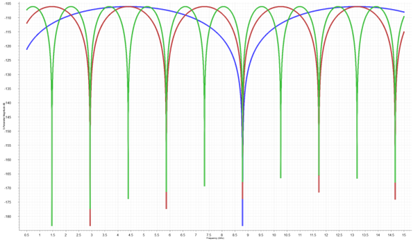
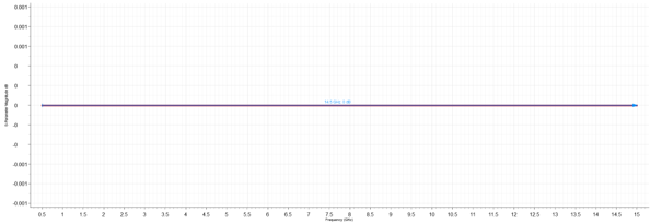
What stands out immediately when comparing S₁₁ and S₂₁? S₁₁ is extremely small for all three line lengths, while S₂₁ remains at 0 dB throughout.

Since the lines are ideal and lossless, the input signal is not attenuated. It therefore arrives at the output entirety. Therefore the magnitude of S₂₁ remains at 0 dB regardless of the line length.

The behavior of S₁₁ can also be explained by the ideal matching. Both the ports and the transmission lines do have an impedance of 50 Ω. Consequently, there are no impedance mismatches at the junctions where the signal could be reflected. Theoretically, S₁₁ therefore equals zero. In the logarithmic representation, this corresponds to a value of −∞ dB.

In the simulation, the S₁₁ values shown are mostly below −100 dB. Such values are practically irrelevant and can be considered as residual numerical quantities from the calculation.

Nevertheless, the waveforms differ significantly. As the TL length increases, the narrow dips occur more frequently. For the 10-mm line, only one pronounced dip is visible, while the pattern repeats more frequently for the 30-mm and 60-mm cables.

However, these dips are not indicative of problematic resonances. In an ideal and fully matched line, S₁₁ would theoretically be −∞ dB across the entire frequency range. The simulator cannot accurately represent this ideal value and instead calculates very small residual values. Their behavior is influenced, among other factors, by the electrical length and the associated phase.

For a practical evaluation, therefore, it is not the number of dips that is decisive, but rather the overall extremely low level of S₁₁. All three lines are equally well-matched. In this ideal model the longer line exhibits neither higher reflections nor greater transmission losses.

This highlights the obvious relationship: If virtually no energy is reflected and the TL shows no losses, the signal reaches the output without attenuation. Accordingly, S₁₁ is at a very low level, while S₂₁ remains at 0 dB.

In the next experiment, the line length remains unchanged, instead, we vary the characteristic impedance value of the ideal TL:

• 30 Ω – blue
• 50 Ω – red
• 75 Ω – green

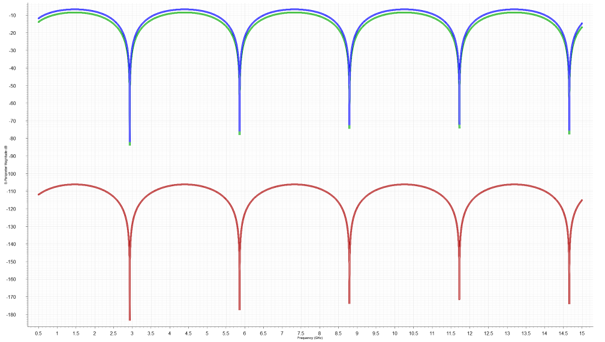
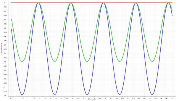
The red 50-Ω waveform continues to show the behavior of an ideally matched line, hence S₁₁ remains extremely small and S₂₁ is 0 dB. But, the 30-Ω and 75-Ω lines behave quite differently.

Since their impedance differs from the reference impedance of the ports, reflections do occur at the junctions. As a result, S₁₁ increases while S₂₁ decreases at the same time. Thus, part of the input energy does not arrive at output ports, it is reflected back to the input port.

The periodic behavior of S₁₁ and S₂₁ is remarkable. This is caused by the electrical length of the mismatched line. Since the electrical length changes with frequency, the impedance at the output—as seen at the line’s input—also changes.

If the electrical length of the line corresponds to half a wavelength or a multiple of them, the input once again sees the 50-Ω termination with the mismatched line. This results in fewer reflections: S₁₁ reaches a minimum and S₂₁ approaches 0 dB.

In contrast, when the length is an odd multiple of a quarter-wavelength, the termination impedance is transformed significantly. The mismatch at the input is then at its highest value: S11 increases and S21 decreases accordingly. As the frequency increases, this behavior will repeat, resulting in the wave-like shape of the S-parameter.

For this reason, S₁₁ reaches very low values at certain frequencies, even though the line impedance still does not match the 50-Ω system. A single deep dip in the S₁₁ curve therefore does not automatically mean that the line is well-matched across the entire frequency range. What truly matters is the shape of the entire waveform.

This relationship is also evident in S₂₁. As S₁₁ increases, S₂₁ decreases. If larger portions of the signal energy will be reflected, correspondingly less energy arrives at the output. As reflection decreases, S₂₁ approaches 0 dB again.

With the 30-Ω line, the deviations are somewhat more noticeable than with the 75-Ω line. It deviates slightly more from the reference impedance of 50 Ω and therefore produces larger reflections. This is evident both in the higher S₁₁ level and in the deeper dips in S₂₁.

Since the lines remain ideal and lossless, no power is lost due to conductor or dielectric losses. The injected power is either transmitted to the output or reflected back to the input. This is why the S21 level remains constant even as the frequency increases.

3. From an Ideal Transmission Line to a Real PCB-Microstrip Structure

Now as we have examined the principles of ideal lines, we will turn our attention to the practical aspect: A microstrip-line structure on a printed circuit board.
With an ideal line, we could simply set for an analysis using a simulator the characteristic impedance to 30 Ω, 50 Ω, or 75 Ω. With a real microstrip line, however, this value is determined by the geometry of the PCB structure and the electrical properties of the material used.

There are three key parameters that can significantly affect the characteristic impedance:

• the trace width “w” ,
• the distance to the reference plane “h” ,
• the relative permittivity or dielectric constant “ε” _”r” .

Why is this important for the resulting S-parameters? If the characteristic impedance will change due to changing one (or multiple) of these parameters, the transmission line may no longer match the 50-Ω system. Reflections will occur at the transitions, which are reflected and represented in S₁₁. At the same time, less energy is transmitted to the output, which also changes S₂₁.

Which factors primarily determine the energy losses? These include the material loss tangent tan(φ) and the conductivity σ of the copper. A higher loss tangent causes higher dielectric losses. Lower copper conductivity increases conductor losses. Both effects result in a higher attenuation and less energy arrive at the output.

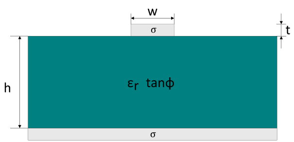
Other factors that influence the behavior include the etching factor and the copper layer thickness. However, their effects are treated as negligible in these experiments

But what effect does the transmission line length have? The length does not change the characteristic impedance of a uniformly constructed microstrip line at all. However, it does affect the propagation time and phase. Due to material losses, it also affects the total signal attenuation. A longer transmission line therefore exhibits greater losses in S₂₁ than a shorter one.

In the following simulation experiments, we will change the individual TL layout and material parameters one at a time. Our goal is to see how a change in the layout structure will be reflected in S₁₁ and S₂₁ and what conclusions can be taken from this for the practical evaluation of a trace behaviour on a PCB.

4. The Effect of the Trace Width

As the first practical parameter we perform a variation of the trace width w. We begin with a 30-mm-long microstrip line designed for 50Ω. We then only vary the trace width until the characteristic impedances becomes 30Ω and 75Ω accordingly. All other geometrical and material parameters remain unchanged. It should be noted that it is quite difficult to design impedances with such an exact precision using realistic design-parameters, hence a tolerance of ±0.2Ω must be assumed at minimum

Here the general impedance/track width rule applies: The wider the trace, the lower its characteristic impedance, the narrower the trace, the higher its characteristic impedance will be.

The following variants were considered for the simulation:

• 30Ω – blue: wide trace
• 50Ω – red: adjusted trace width
• 75Ω – green: narrow trace

The ports continue to have a reference impedance of 50 Ω.

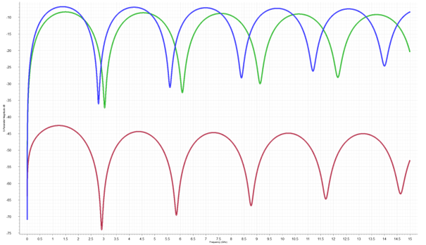
The red 50-Ω line exhibits the lowest reflections across the entire frequency range. Its trace width is designed so that its characteristic impedance is nearly equal to the reference impedance of the two 50-Ω ports. As a result, only very small reflections do occur at the transitions.

In contrast, for the 30-Ω and 75-Ω lines the characteristic impedance does not match the reference impedance. This is due to the different trace widths. Consequently, a larger portion of the signal is reflected at the transitions between the port and the line, causing S₁₁ to increase significantly.

However, the deep dips in the S₁₁ curves do not mean that the lines suddenly have a characteristic impedance of 50 Ω at these frequencies. The trace geometry—and thus its characteristic impedance—remains unchanged. Instead, the line transforms the 50-Ω termination depending on its electrical length. At certain frequencies, the input impedance thus appears nearly matched to the 50-Ω system, causing S₁₁ to reach a minimum.

The 30-Ω line shows stronger reflections than the 75-Ω line. The decisive factor here is not merely the delta to the reference impedance, but the ratio of the two impedances. Consequently, the transition from 50 Ω to 30 Ω results in a higher reflection coefficient than the transition from 50 Ω to 75 Ω. Accordingly, the blue S₁₁ curve reaches higher values than the green one.

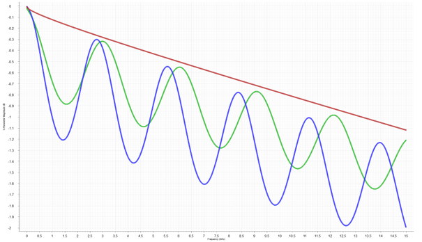
For the 50-Ω line, S₂₁ remains relatively constant and decreases slowly as the frequency increases. This is caused by the loss in the copper and in the dielectric. Unlike an ideal transmission line investigated in the beginning, S₂₁ does not exactly equal 0 dB even with a good matching. A portion of the signal energy will be converted into heat due to conductor and dielectric losses while travelling to the output.

In the case of the 30-Ω and 75-Ω transmission lines, a significant ripple is added to the general attenuation. This is caused by the mismatch to the 50-Ω system. If S₁₁ is large, a larger portion of the signal energy is reflected and S₂₁ drops more sharply as a result. At frequencies where the input impedance is transformed closer to 50Ω by the line, reflection decreases and S₂₁ again approaches to the behavior of a matched transmission line. This illustrates the relationship between the two S-parameters: If reflection increases due to a mismatch, less signal energy reaches the output.

5. The Effect of the Distance to the Reference Plane

Next, we will examine the impact of the distance h between the trace and the reference plane. Once again, we begin with a 30-mm-long microstrip line designed for a characteristic impedance of 50Ω.

We then vary only the distance to the reference plane until characteristic impedances of approximately 30Ω, 50Ω and 75Ω are achieved. All other geometric and material parameters remain unchanged.

As a general rule: The smaller the distance to the reference plane, the lower the characteristic impedance of the transmission line. The greater the distance, the larger the characteristic impedance.

The following variants have been considered for the simulation experiments:

• 30Ω – blue: small distance from the reference plane
• 50Ω – red: initial condition
• 75Ω – green: larger distance from the reference plane

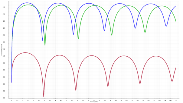
This behavior essentially corresponds to the previously observed effect of trace width change. Here also the red 50-Ω trace exhibits the smallest reflections, while the 30-Ω and 75-Ω traces show significantly higher S₁₁ values due to mismatch.

The trend visible in the S-parameters differs only slightly from the results of the previous experiment. This time, the root cause of the impedance change is not the trace width, but the distance to the reference plane.

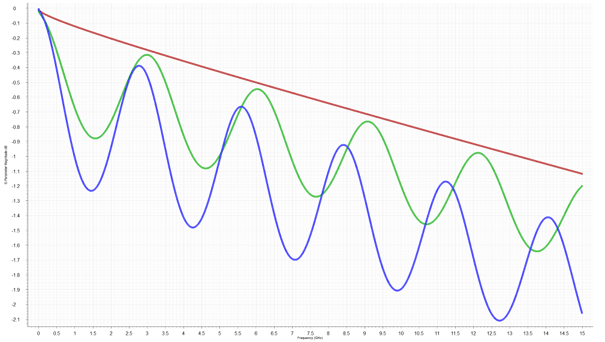
The same behavior is also evident for S₂₁. The matched 50-Ω line exhibits a relatively smooth response. For the 30-Ω and 75-Ω lines, significant ripple is added to the normal line attenuation. As S₁₁ increases, S₂₁ decreases more sharply since a larger portion of the signal energy will be reflected.

Compared to the variation of the trace width, the S-Parameter curves differ only slightly. The magnitudes of S₁₁ and S₂₁,  are rather identical: The 50-Ω line is well-matched, while the 30-Ω and 75-Ω lines exhibit significantly stronger reflections.

The reason for this is that the S-parameters primarily reflect the effects of the resulting characteristic impedance. Whether a 30-Ω line is created by a wider trace width or by a smaller distance to the reference plane is of secondary importance for the reflection at the 50-Ω port. In both cases, the signal exhibits a line with the same characteristic impedance.

This is precisely where the “aha” moment occurs: The S-parameters clearly show that a mismatch is present. However, the curves alone do not clearly indicate which layout parameter caused this mismatch.

Small differences are nevertheless visible. The positions of the maxima and minima may shift slightly and the attenuation may also differ to a certain extend. The change in the distance to the reference plane alters the field distribution, the effective permittivity and thus the signal propagation speed.

This means for a practical analysis that slight changes to the PCB track design may produce very similar S-parameters if they result in a close characteristic impedance range.

6. The Effect of the Dielectric Constant

Finally, we will examine the relative permittivity , often referred to as D_k. Once again, we start with a 30-mm-long microstrip line designed for a characteristic impedance of 50Ω.

We then vary only D_k until characteristic impedances of approximately 30Ω, 50Ω, and 75Ω are achieved. All other geometrical and material parameters will remain unchanged.

Generally: If the dielectric constant increases, the characteristic impedance of the TL will decrease. Conversely, a lower D_k value results in a higher characteristic impedance.

To change the characteristic impedance significantly solely through D_k, comparatively large changes in material properties are required. This shows that while D_k does influence the characteristic impedance, in practice it can only be used to a limited extent as a control variable. In most cases, the base material is already selected based on other requirements (manufacturing, availability, costs), while the impedance is subsequently adjusted primarily through the trace geometry.

For the simulation, the three familiar cases arise again:

• 30Ω – blue: high D_k
• 50Ω – red: initial condition
• 75Ω – green: lower D_k

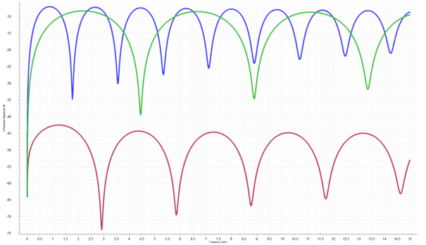
In this experiment also the 50-Ω line exhibits the lowest reflections, since its characteristic impedance matches the reference impedance of the ports best. In contrast, the 30-Ω and 75-Ω lines result in a mismatch, causing S₁₁ to increase significantly.

Compared to the previous experiments an additional effect is noticeable: the position/frequency of the maxima and minima do change more significantly. When varying the trace width or the distance from the reference plane, the S-Parameter curves were still largely similar in their behavior. A change in D_k, on the other hand, affects not only the characteristic impedance but also the signal propagation speed. More specifically, the effective dielectric constant of the microstrip line changes. As D_k increases, the signal propagates slower. As a result, the line becomes electrically longer while maintaining the same physical length and the maxima and minima of the S-Parameters occur at lower frequencies or more frequently within the frequency range under consideration. With a smaller D_k, the opposite is the case.

The key difference is therefore: When D_k changes, the S-parameters reflect not only the effects of a varying impedance. At the same time, the electrical length of the line also changes, which is evident in the shift visible in the curves.

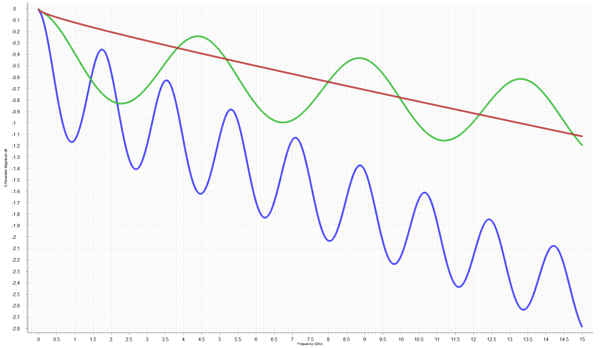
The basic pattern is also evident in S₂₁: The 50Ω line exhibits the smoothest response, while the 30Ω and 75Ω lines show significant ripples due to mismatch.

Compared to the previous geometric changes the differences are more pronounced this time. Particularly for the 30Ω line, the attenuation S₂₁, increases significantly as the frequency rises. Thus, the curve not only becomes more undulating but also deviates increasingly from the profile of the matched 50Ω line. This effect is also visible for the 75Ω line, though it is less pronounced.

And this is the insight behind these results: A change in D_k affects not only the characteristic impedance but also the propagation of the signal. As the dielectric constant increases, the propagation speed decreases, causing the line to become electrically longer while maintaining the same physical length. This is why the maxima and minima shift significantly, unlike when varying the trace width or the distance from the reference plane.

Depending on the used material, the dielectric losses may also change. This can cause S₂₁ to drop even further. However, a higher D_k does not automatically mean higher losses; the loss factor of the material is the dominant factor here.

The S-parameters thus reliably indicate that the transmission characteristics of the TL have changed. However, the S-Parameters itself do not allow a clear determination of which material or layout parameter is responsible for what kind of ‘misshaping’ in the waveform. To do so, the underlying geometry and material data must also be considered.

7. Conclusion and Outlook

The simulation-experiments lead to one general conclusion: Most changes to a microstrip line will be reflected directly in the S-parameters, mainly via the characteristic impedance effect.

If the transmission line is well-matched to a 50-Ω system, S₁₁ remains low. The behavior of S₂₁ is then determined primarily by the actual conductor and the dielectric losses. If on the other hand, the characteristic impedance deviates from 50 Ω, reflections will occur. S₁₁ increases and additional dips and ripples appear in S₂₁.

However, the curves alone cannot clearly reveal the root cause of such a mismatch. An inappropriate trace width, a changed distance to the reference plane or a different dielectric material constant can nevertheless create the same characteristic impedance and thus lead to very similar S₁₁ and S₂₁ curves.

And this is important to mention: The S-parameters can reliably indicate that the transmission characteristics have changed along the path from driver to (the) receiver(s). However, they cannot directly reveal which layout- or material-parameter is responsible for this. For a definite assessment, the layer-stack up, the trace geometry and the material properties must therefore also be taken into account.

The comparison with the ideal transmission line also underlines the effects occurring in a real microstrip line. Even a well-matched 50-Ω line does not transmit the signal completely lossless. As the frequency increases, losses in the copper and the dielectric cause S₂₁ to continue to decrease.

All simulations in this contribution have been performed using the Zuken SI-Simulator in its frequency domain simulation mode (this simulator is available as add-on in Zuken CR-8000 and eCADSTAR products).

In this manner, simulation is not only a tool for verifying a finished PCB layout, it helps to better understand the inter-relationships on a printed circuit board. When individual parameters are specifically modified and the resulting S-parameters are compared, the effects of a layout decision become immediately apparent.

However, this is only the first small step in answering all such questions. In further investigations the loss factor of the PCB material or the conductivity of the copper or the influence of propagation time, phase, and electrical length could be examined in greater detail. Equally interesting would be the question of how a 50Ω trace is specifically dimensioned and at what trace length-controlled impedance actually becomes relevant.

Which of these topics should be the focus of our next post? Let us know in the comment section below!