
Preparing S-parameters/Touchstone® Model for High-Speed PCB Analysis
In past years, more design engineers started to use S-parameters/Touchstone® for Signal Integrity and Power Integrity analysis. The S-parameters/Touchstone® is nothing new. However, it is becoming more popular because it covers good information in a simplified behavioral format. Still, it does have some disadvantages if a lack of data accuracy or/and sufficiency is present.
In this post, I’ll introduce the history and content of S-parameters/Touchstone®. We also will discuss its advantages and disadvantages and how to use the tool to overcome the issues.
History of S-parameters
S-parameters refer to the scattering matrix of a microwave network; the “S” in S-parameters refers to scattering.
Before the 1950s and the extensive use of high-frequency systems, network parameters like Y- and Z-parameters were the primary method of characterizing circuit performance. At higher frequencies, the concept of voltages and currents became more difficult to relate to network performance – especially in networks using transmission lines like waveguides. S-parameters are related to power waves and eliminate many of these issues.
The 1948 Radiation Laboratory series, “Principles of Microwave Circuits,” introduced the emerging microwave community to practical approaches to solving microwave design problems using scattering parameters in the design of circuits.
It helped that during the 1960s, Hewlett Packard introduced the first microwave network analyzers. The scattering wave concept was further popularized around the time that Kaneyuki Kurokawa of Bell Labs wrote his 1965 IEEE article “Power Waves and the Scattering Matrix.” Also, Robert Collin’s textbook, Field Theory of Guided Waves, published in 1960, has a brief discussion on the Scattering matrix. Collin’s book is extensively annotated, including an author index, which reads like a Who’s Who of electromagnetic theory for the first half of the twentieth century.
The word “Touchstone” was issued by EEsof (a part of Agilent Technologies, now Keysight). In 2009, Touchstone 2.0 was ratified by IBIS. Touchstone 2.0 added resistance per port option for Power Delivery System and mixed-mode features for differential setups. Currently, Touchstone 1.0 is widely supported by most of the tools. Touchstone 2.0 is still not supported by a number of EDA vendors.
Contents of S-parameters
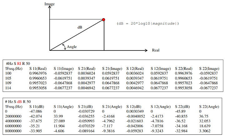
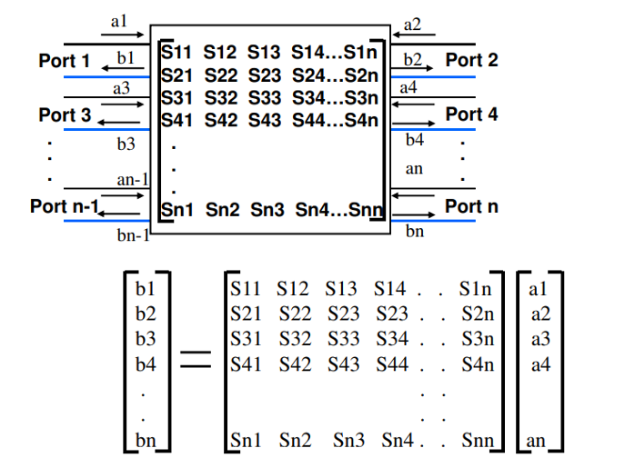
What do the S-parameters contain? An S-parameters model contains the information for the gain/loss and phase against reference resistance port(s) on the frequencies.
Original S-parameters and Touchstone 1.0 only allow the single reference port for one model, but Touchstone 2.0 enables multi-reference ports in an S-parameters model.
- 2-port and n-port S-parameter/Touchstone® format and contents are shown below:
- 2-port:
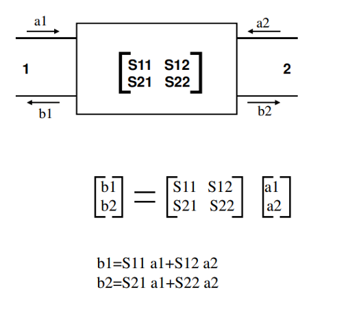
-
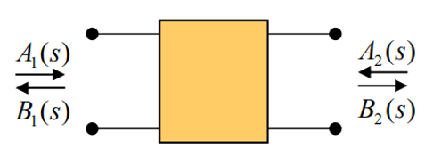
- N-port:
Strengths and Weaknesses when Using S-parameters in Analysis
S-parameters are used more and more in high-speed digital circuit designs, so it’s not new to SI/PI engineers. But why are S-parameters used often in SI/PI analysis in multi-GHz channel analysis?
Consider these reasons:
- S-parameters are always defined, though impedance or admittance may not be.
- S-parameters are normalized. There are good numerical properties in the simulations.
- S-parameters are easily measured, even at very high frequency. Better for simulation and measurement correlations.
- Standardized format for S-parameters (Touchstone®). The measurement equipment uses Touchstone® for output. Most field solvers provide Touchstone® output as well.
- Tabulated ASCII format frequency data does not disclose any design details but only electrical properties.
- The best way to represent broadband EM/circuit interactions. It is the essence of Signal and Power Integrity.
With a lot of advantages from S-parameters, there are also some weaknesses in simulations when S-parameters data has:
- Limited frequency range coverage
- DC point absent
- Coarse sampling
- Unintentional non-passivity
- Measurement noise
Effects of Passivity and Causality Issues in S-parameters/Touchstone®
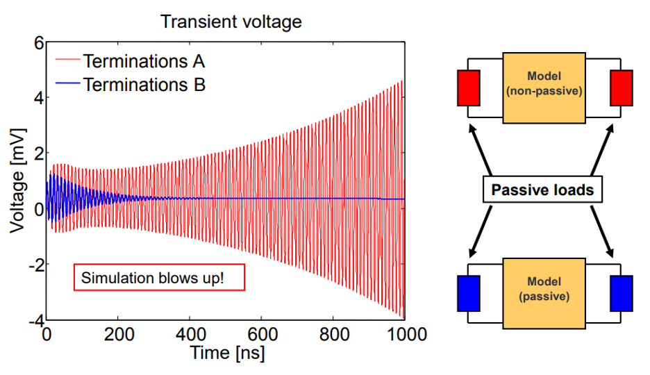
- Passivity
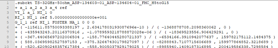
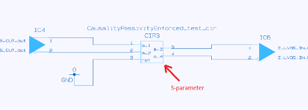
In passive interconnects, such as traces, vias, wires, etc., the signal from one end to another should not have gained. Instead, it should always have a loss. S-parameters/Touchstone® is designed for passive elements. The simulation will be “exploded” if the S-parameters/Touchstone® model is not passive. See the image below.
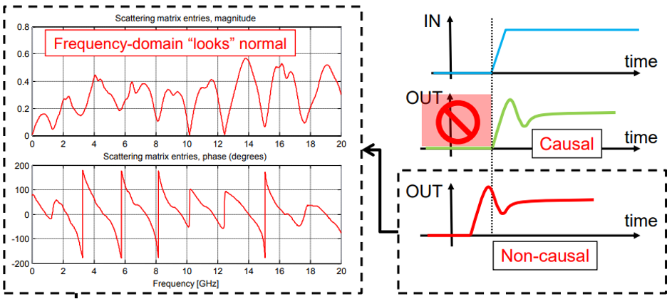
- Causality
- When a signal goes through a passive interconnect from one end to another, the input signal will always be earlier than the output signal. Given that the S-parameters/Touchstone® file is frequency-oriented, sometimes we find the output signal is earlier than the input signal in time-domain simulations. This is called a non-causal event. Non-causal events directly affect channel analysis accuracy, especially for timing analysis. The picture below shows what a non-causal event is.
Preparing S-parameters/Touchstone® for SI/PI Simulations
We discussed that S-parameters/Touchstone® has many advantages for SI/PI analysis. And we also know it is not a silver bullet. To optimize its advantages, we need to minimize its disadvantages by checking and fixing the possible issues that S-parameters/Touchstone® might have before using it in SI/PI simulations.
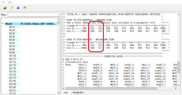
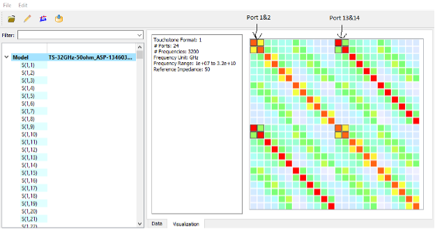
Many EDA tools support S-parameters/Touchstone® models for SI/PI simulations. Here, I use a 24-pin connector (S24P) S-parameter/Touchstone® 1.0 model (93.6 MB, 461060 lines) as an example to describe how Zuken’s CR-8000 tools support S-parameters/Touchstone® model for simulations.
Step 1: Load into the simulation library
At the beginning of the model file, the comments show P01 connects to P13 and P02 connects to P14 as circled in RED from the visual checker. We will focus on these four pins to find out how to check the data and import these pins only into the library to save the file size.
Step 2: Visualization check
The tool’s visualization checking feature provides a visual representation of insertion losses and data symmetrical arrangements. It also visually highlights data if it is out of range in the S-parameters/Touchstone® model files.
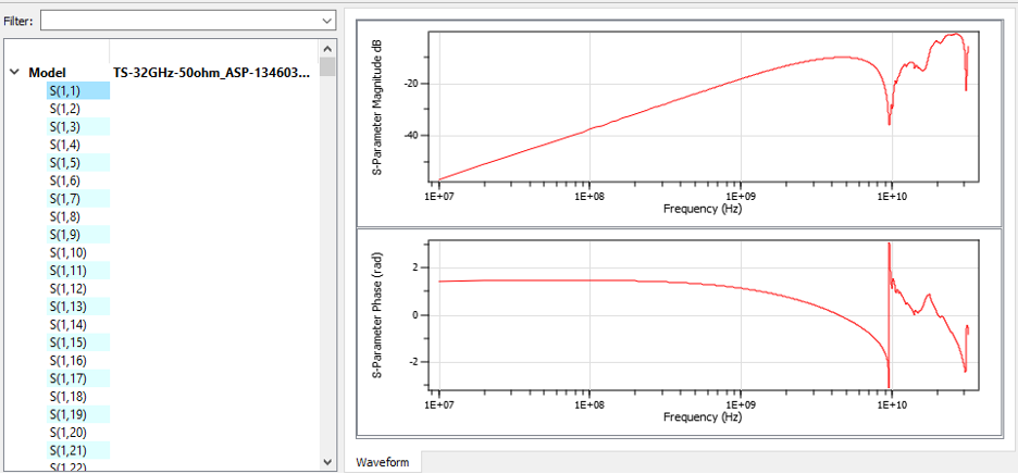
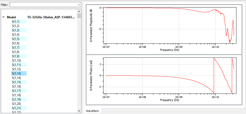
Step 3: Check the data for each frequency response
S(1, 1): Reflections
S(1, 13): Insertions
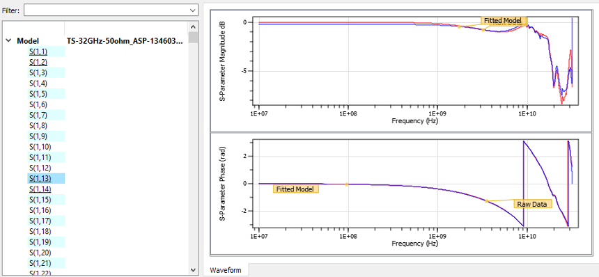
Step 4: Extracting and fitting
Most of the time, we only focus on specific ports inside a large S*P file to reduce the file size and simplify the fitting process. In this case, we have a huge S24P file (93.6MB). To start, we will extract only four ports (Port 1, 2, 13, and 14) for our differential pair simulations.
We take ports 1, 2, 13, and 14 as “only selected” ports to extract and convert to the SPICE netlist for future simulations.
In Zuken tools, “Direct pole-residue specification” is used for the conversions.
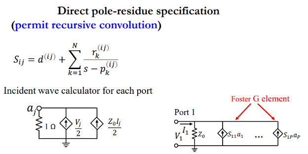
In the import assistant dialog, we can define the accuracy settings for fitting as well as passivity, reciprocity and causality enforcements before fitting and passivity enforcement after fitting. It also offers lowpass off band behavior enforcement and DC extrapolation in case it is needed.
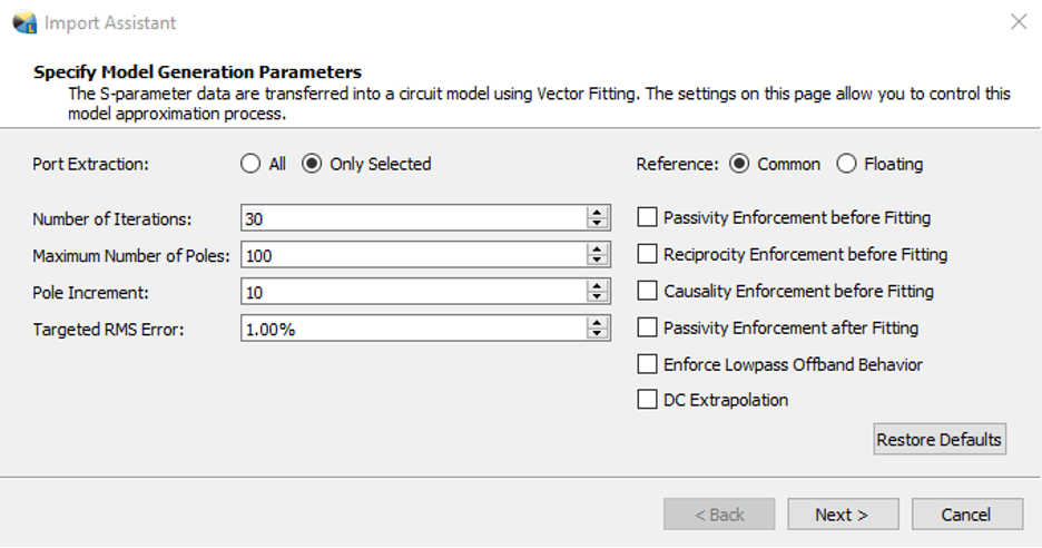
We skip all the enforcement features for the first run of conversion.
S(1, 1):
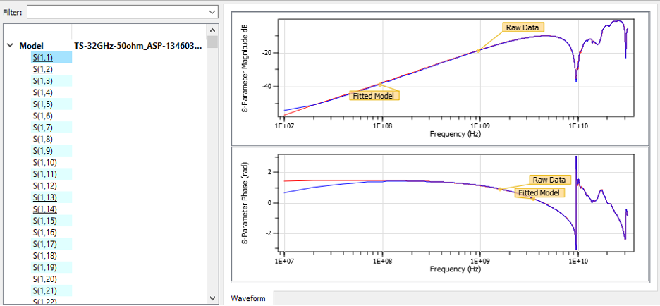
S(1, 13):

From the results, we can see the fitted data are well-aligned with the original data except in the low-frequency area (< 100MHz)
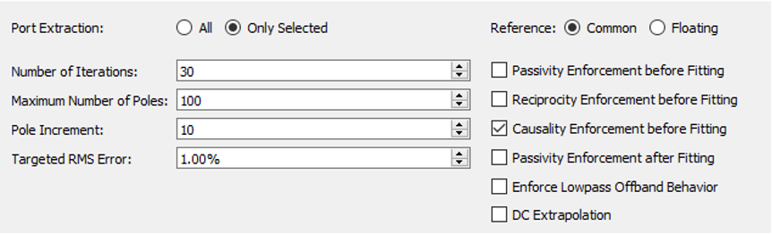
Step 5: Tests for causality enforcements and DC extrapolation
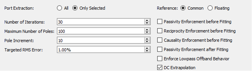
- The test with causality enforcement only
In the result shown below, the original data and the fitted data for S(1, 13), the part of insertion loss, pretty much agreed with each other. However, the original data and the fitted data for S(1, 1), the part of reflection, have some disagreements, especially for the low-frequency range. In other words, the reflection part of this model needs to be fixed for non-causal conversions.
S(1, 1):
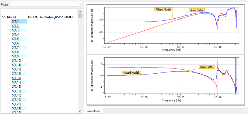
S(1, 13):
- The test with DC extrapolation only
- As the results show below, both S(1, 1) and S(1, 13) mostly agree between the original and fitted data. We can tell that the data for DC and low-frequency area is sufficient in this S-parameters/Touchstone® file.
S(1, 1):
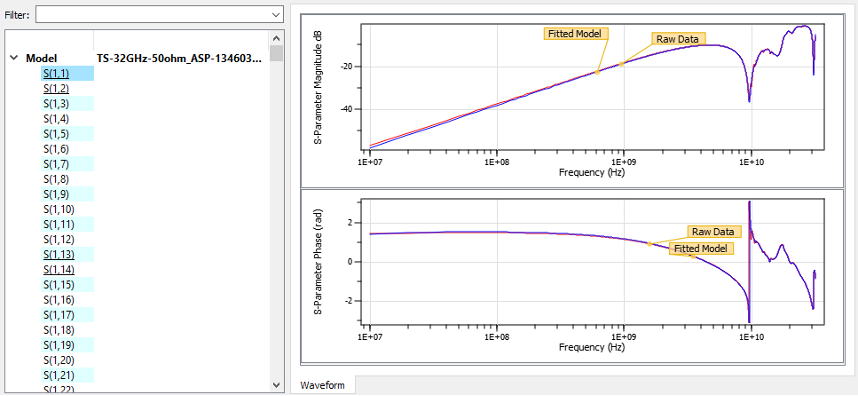
S(1, 13):
Step 6: Simulation with fitted models
After pole-residue conversions, the fitted model stored in the library is in broadband SPICE format.
It can be used as an N-port SPICE circuit for simulations. If the common reference is selected, it will contain only one reference node; if the floating reference is selected, each port will have a reference node separately. It is essential to connect the proper reference node(s) for accurate simulation results.
Conclusions
S-parameters/Touchstone® is very useful for multi-GHz high-speed channel analysis. Touchstone 2.0 is also an international standard ratified by IBIS Open Forum. It is easily used with measurement correlations and frequency responses. It uses a “black box” type ASCII format for greater interoperability and intellectual property protection.
The S-parameters/Touchstone® model is not a silver bullet. It has some weak points, especially if there is a mistake when the model was created. It is not easily found even with visual graphical curve checks. It is not possible to be fixed by hand either. Using a tool (such as Zuken’s CR-8000 Analysis Module) for checking and enforcing is essential to ensure accurate simulation results for SI/PI analysis.
References:
https://www.microwaves101.com/encyclopedias/s-parameters
What You Can Read, What You Have to Read, Shinichi Maeda, KEI Systems, IBIS Summit
Towards Real-time S-parameter qualification and macromodeling, Stefano Grivet Talocia, Politecnico di Torino, Italy, IBIS Summit
Optimum Frequency Sampling in S Parameter Extraction and Simulation, Jinhua Huang, Synopsys, China, IBIS Summit
Overcoming Signal Integrity Channel Modeling Issues | Signal Integrity Journal, John Baprawski, SerDes Systems, Signal Integrity Journal
Circuit Synthesis of Multiport Networks from Passive Poles and Residues, Chiu-Chih (George) Chou & José E. Schutt-Ainé, DesignCon IBIS Summit 2022
S-parameter Renormalization, The Art of Cheating | 2017-01-12 | Signal Integrity Journal, Gustavo Blando, Oracle Co. Signal Integrity Journal

- Blog
Modern electronic products are no longer built around a single PCB. As systems become faster, denser, and more interconnected, engineering teams are being forced to rethink how they design, verify, and manage complex multi-board products.
- Blog
Explore how CR-8000 enhances PCB design with integrated control of impedance and resistance—enabling precise analysis for both high-speed and high-power applications, from signal integrity to power distribution optimization.

- Blog

- Blog
AI in PCB design is increasingly seen as a game-changer, with some predicting it could soon replace entire layout teams—but this view risks overlooking both the current limits of AI and the critical expertise engineering demands. At DesignCon 2025, experts from emphasized that AI's real value lies in complementing human judgment, not replacing it. Read more on our blog.
- Blog
Modern electronic products are no longer built around a single PCB. As systems become faster, denser, and more interconnected, engineering teams are being forced to rethink how they design, verify, and manage complex multi-board products.
- Blog
Explore how CR-8000 enhances PCB design with integrated control of impedance and resistance—enabling precise analysis for both high-speed and high-power applications, from signal integrity to power distribution optimization.
- Blog
- Blog
AI in PCB design is increasingly seen as a game-changer, with some predicting it could soon replace entire layout teams—but this view risks overlooking both the current limits of AI and the critical expertise engineering demands. At DesignCon 2025, experts from emphasized that AI's real value lies in complementing human judgment, not replacing it. Read more on our blog.